Isolated dipole farfield

The fmmax.farfield module provides functions that enable the calculation of farfield radiation patterns, e.g. from dipole sources embedded within a stack of thin films. Since the Fourier Modal Method deals with biperiodic structures, such a calculation will generally yield the farfield pattern from a periodic array of dipoles. However, when combined with Brillouin zone integration, one can calculate the farfield radiation pattern of an isolated dipole in the stack. The ability to perform such calculations is useful, e.g. to study the distribution of carriers in a multi-quantum well active region (David et al.).

In this notebook, we demonstrate the use of Brillouin zone integration and the fmmax.farfield module to compute the farfield of an isolated dipole in the simple case of a dipole in vacuum. The same approach can be used to compute the farfield for a dipole in an arbitrary stack of thin films.

Dipole in vacuum

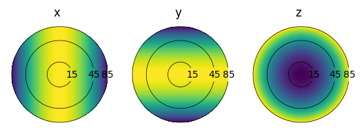
First, we’ll take a look at the farfield pattern from a dipole in vacuum. This is a useful starting point since the farfield pattern can be computed analytically; we can use the analytical expression for the farfield pattern to valdiate the numerical result computed. The analytical expression for farfield intensity is \(I(\gamma) \propto \sin^2(\gamma)\) if \(\gamma\) is the angle with respect to the polarization direction of the dipole.

Next, we’ll compute the farfield pattern numerically. We use a wavelength of 1.0 and choose a unit cell which is smaller than one half wavelength to ensure that only the (0, 0) Fourier order corresponds to a propagating wave. Since we are interested in the farfield, we only need to include the propagating waves in our Fourier expansion. Thus, with such a small unit cell we only need to include a single Fourier order in the expansion.

import numpy as onp
import fmmax

wavelength = onp.asarray(1.0)
pitch = 0.45
primitive_lattice_vectors = fmmax.LatticeVectors(pitch * fmmax.X, pitch * fmmax.Y)
expansion = fmmax.Expansion(onp.asarray([[0, 0]], dtype=int))

We’ll use Brillouin zone integration to model an isolated dipole. To do this, we need to compute the fields using expansions that are centered around wavevectors on a grid in the Brillouin zone; generate the in-plane wavevectors associated with each point on this grid.

in_plane_wavevector = fmmax.brillouin_zone_in_plane_wavevector(
    brillouin_grid_shape=(101, 101),
    primitive_lattice_vectors=primitive_lattice_vectors,
)

We can now solve for the modes of our periodic vacuum and compute its scattering matrix.

import jax.numpy as jnp

solve_result_vacuum = fmmax.eigensolve_isotropic_media(
    permittivity=jnp.asarray([[1.0]]),
    wavelength=jnp.asarray(wavelength),
    in_plane_wavevector=in_plane_wavevector,
    primitive_lattice_vectors=primitive_lattice_vectors,
    expansion=expansion,
)
s_matrix_vacuum = fmmax.stack_s_matrix(
    layer_solve_results=[solve_result_vacuum],
    layer_thicknesses=[1.0],
)

Next, define the sources associated with x, y, and z-oriented dipoles. These are stacked into a single array, with the final axis of the array corresponding to the dipole orientation. This is consistent with the FMMAX convention of using the trailing axis as the batch axis for wave amplitudes and electromagnetic fields.

dipole = fmmax.dirac_delta_source(
    location=jnp.asarray([[pitch / 2, pitch / 2]]),
    in_plane_wavevector=in_plane_wavevector,
    primitive_lattice_vectors=primitive_lattice_vectors,
    expansion=expansion,
)
zeros = jnp.zeros_like(dipole)
jx = jnp.concatenate([dipole, zeros, zeros], axis=-1)
jy = jnp.concatenate([zeros, dipole, zeros], axis=-1)
jz = jnp.concatenate([zeros, zeros, dipole], axis=-1)

Next, we compute wave amplitudes assuming that the dipole source is sandwiched by vacuum layers above and below. We’ll consider the backward-going amplitude in the first layer, which is equivalent to the forward going amplitude in the second layer. Since the only source is between the two layers, the forward going amplitude in the first layer is zero, as is the backward-going amplitude in the second layer.

From the amplitude we compute the flux, i.e. the power in each Fourier order. Again, only the backward flux will be nonzero.

bwd_amplitude_0_end, *_ = fmmax.amplitudes_for_source(
    jx=jx,
    jy=jy,
    jz=jz,
    s_matrix_before_source=s_matrix_vacuum,
    s_matrix_after_source=s_matrix_vacuum,
)
_, backward_flux = fmmax.directional_poynting_flux(
    forward_amplitude=jnp.zeros_like(bwd_amplitude_0_end),
    backward_amplitude=bwd_amplitude_0_end,
    layer_solve_result=solve_result_vacuum,
)

Now, compute the farfield profile.

import matplotlib.pyplot as plt

(
    polar_angle,
    azimuthal_angle,
    solid_angle,
    farfield_flux,
) = fmmax.farfield_profile(
    flux=-backward_flux,
    wavelength=wavelength,
    in_plane_wavevector=in_plane_wavevector,
    primitive_lattice_vectors=primitive_lattice_vectors,
    expansion=expansion,
    brillouin_grid_axes=(0, 1),
)
# Sum the s and p polarizations for each direction
farfield_flux = jnp.sum(farfield_flux, axis=-2)
mask = ~jnp.isnan(farfield_flux)
farfield_flux /= jnp.amax(farfield_flux[mask])


def plot_farfield(flux, polar_angle, azimuthal_angle):
    x = jnp.sin(polar_angle) * jnp.cos(azimuthal_angle)
    y = jnp.sin(polar_angle) * jnp.sin(azimuthal_angle)

    for i, orientation in enumerate(["x", "y", "z"]):
        ax = plt.subplot(1, 3, i + 1)
        mask = ~onp.isnan(flux[..., 0])
        ax.tricontourf(x[mask], y[mask], flux[..., i][mask], levels=100)
        for angle_deg in [15, 30, 45, 60, 75, 90]:
            t = jnp.linspace(0, 2 * jnp.pi)
            xa = jnp.cos(jnp.deg2rad(angle_deg)) * jnp.cos(t)
            ya = jnp.cos(jnp.deg2rad(angle_deg)) * jnp.sin(t)
            ax.plot(xa, ya, "k", lw=0.5)
        ax.set_aspect("equal")
        ax.axis(False)
        ax.set_title(orientation)


plot_farfield(farfield_flux, polar_angle, azimuthal_angle)

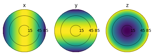
We can also compare this to the analytical farfield.

x = jnp.sin(polar_angle) * jnp.cos(azimuthal_angle)
y = jnp.sin(polar_angle) * jnp.sin(azimuthal_angle)
z_flux = jnp.sin(polar_angle) ** 2
x_flux = jnp.sin(jnp.arccos(x)) ** 2
y_flux = jnp.sin(jnp.arccos(y)) ** 2
analytical_farfield_flux = jnp.stack([x_flux, y_flux, z_flux], axis=-1)

plot_farfield(analytical_farfield_flux, polar_angle, azimuthal_angle)

These are in excellent agreement. Finally, we can plot a cut through the farfield profile, and verify that it has \(cos^2\) dependence.

d = farfield_flux.shape[0] // 2
theta_deg = (
    jnp.rad2deg(polar_angle[:, d])
    * jnp.where(azimuthal_angle[:, d] > -0.9 * jnp.pi, 1, -1)
)

plt.figure(figsize=(6, 2))
ax = plt.subplot(131)
ax.plot(theta_deg, jnp.cos(jnp.deg2rad(theta_deg))**2, lw=6)
ax.plot(theta_deg, farfield_flux[:, d, 0], lw=2)
ax.set_title("x")
ax.set_xlabel("Polar angle")
ax.set_ylabel("Intensity")

ax = plt.subplot(132)
ax.plot(theta_deg, jnp.cos(jnp.deg2rad(theta_deg))**2, lw=6)
ax.plot(theta_deg, farfield_flux[d, :, 1], lw=2)
ax.set_title("y")
ax.set_yticklabels([])
ax.set_xlabel("Polar angle")

ax = plt.subplot(133)
ax.plot(theta_deg, jnp.sin(jnp.deg2rad(theta_deg))**2, lw=6, label="analytical")
ax.plot(theta_deg, farfield_flux[:, d, 2], lw=2, label="numerical")
ax.set_title("z")
ax.set_yticklabels([])
ax.set_xlabel("Polar angle")
_ = ax.legend(bbox_to_anchor=(1, 1))